These models are on purpose somewhat artificial: that makes them simple to understand and to explain. Real world models are often more messy.
In most cases the date sets were developed to show the performance of special purpose algorithms. The current crop of state-of-the-art LP and MIP solvers can solve these problem remarkably efficiently.
option mip=gurobi; |
|
|
This is a fairly small but difficult MIP model. In 1998 the model was largely too difficult to solve to optimality. With current state-of-the-art MIP solvers and multi-core PC's, we can solve this model in about 10 minutes. |
|
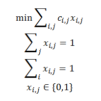
This is a fairly large assignment problem. With Cplex you can use the network optimizer to solve this
very fast. Otherwise standard LP solvers also do a very good job on this, especially compared to a
textbook implementation of the Hungarian Method. Although the assignment problem is stated as a MIP, we solve as an RMIP as the binary variables assume integer values in the optimal solution automatically. As this is a network problem, it may be beneficial to select a network optimizer if available. |
|
|
This is a standard benchmark model that was unsolvable for 25 years. Nowadays it can be solved with standard MIP solvers. This formulation is originally from Alan Manne. |
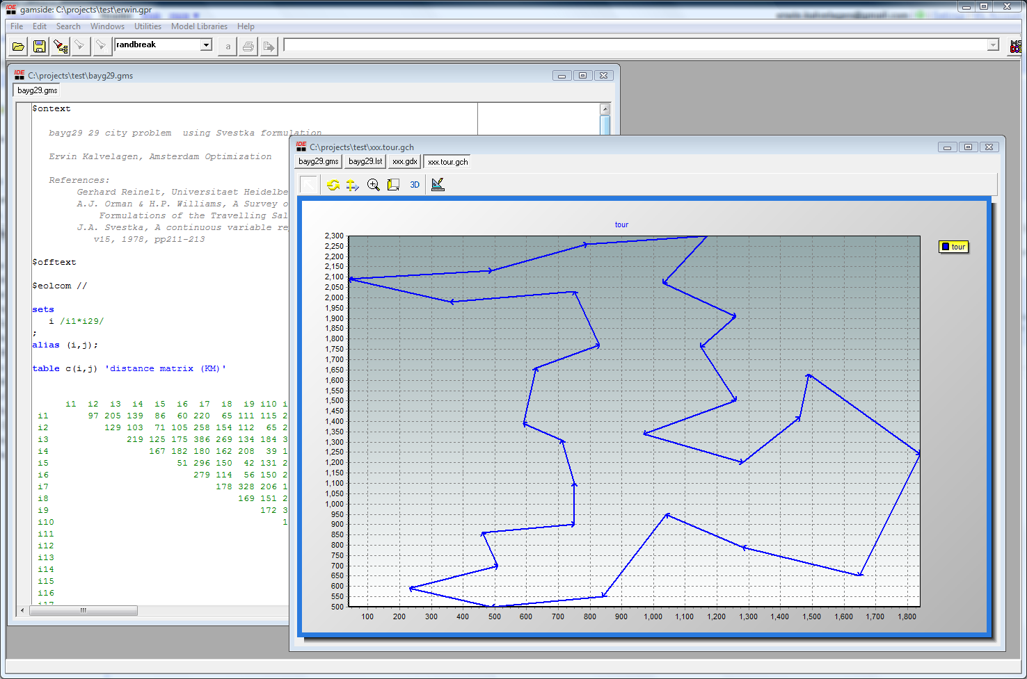
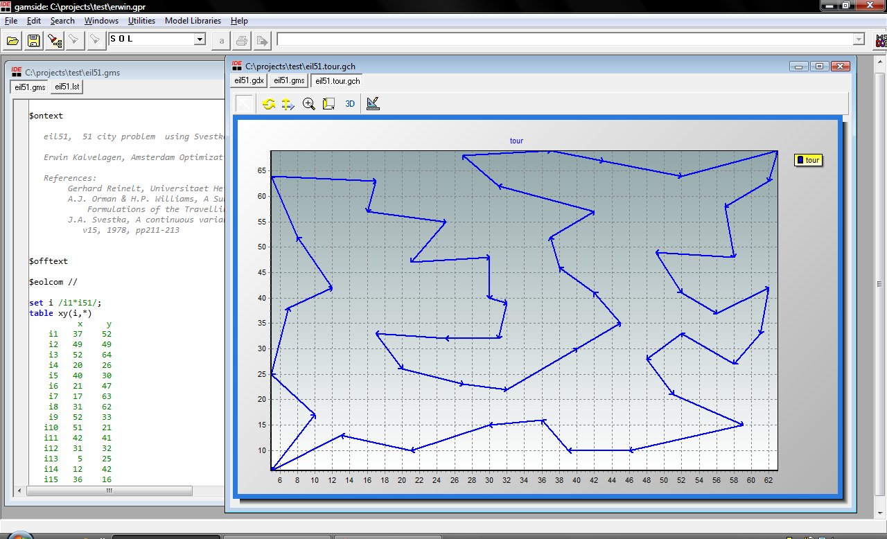
| TSP models are notoriously difficult when solved as a straight MIP. The best MIP solvers can solve problems with about 50 cities. For larger instances we can formulate more specialized algorithms in GAMS. |
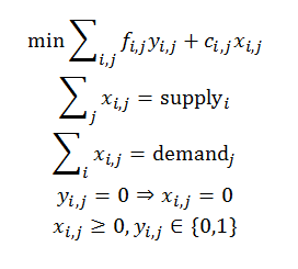
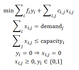
This is a large instance of the capacitated warehouse location problem.
First run whouselocdata.gms to generate capa.inc.
Some Perl code is used to convert the data to GAMS input format.
|
|
|
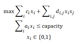
This is a large instance of the Quadratic Knapsack Problem problem.
First run qkpdata.gms to generate qkp.inc.
Some Perl code is used to convert the data to GAMS input format. The model linearizes the
multiplication of binary variables xixj so we can solve
the model with a standard MIP solver.
|
This model was developed to demonstrate an issue with second derivatives in GAMS. It is based on a user model that showed poor performance. The "fast" version shows good performance with some of the interior point codes.
|
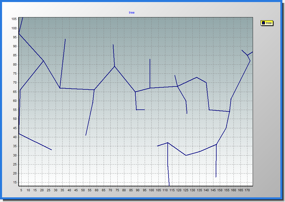
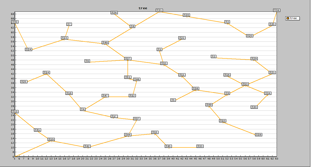
The problem of finding a minimum spanning tree can be formulated as a large LP. |
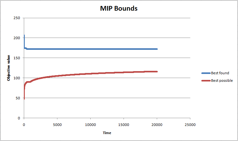
| This is a model with only 4 equations. Good MIP solvers can find very good solutions very quickly, but proving optimality takes a very long time. |
|
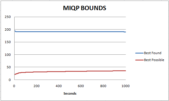
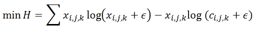
This MIQP model is quite difficult. It finds a permutation matrix such that the
Frobenius norm describing the difference between two matrices is minimized.
It is possible to form a linear assignment problem with the same solution.
A good MIQP solver will be able to find near-optimal solutions very quickly but
proving optimality is very time-consuming.
|
|
 |
 |
|
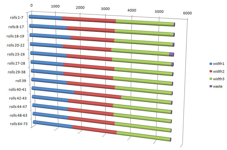
These are tough little models (only 26 rows by 72 or 73 columns) that take a lot of time to
solve to optimality. Especially data set 2 is very difficult.
|
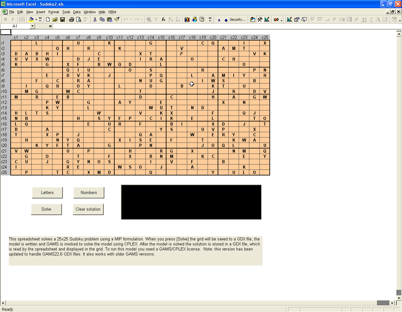
The best MIP solvers can solve these large Sudoku instances completely in the presolve. The iteration count will then be zero.
|
|
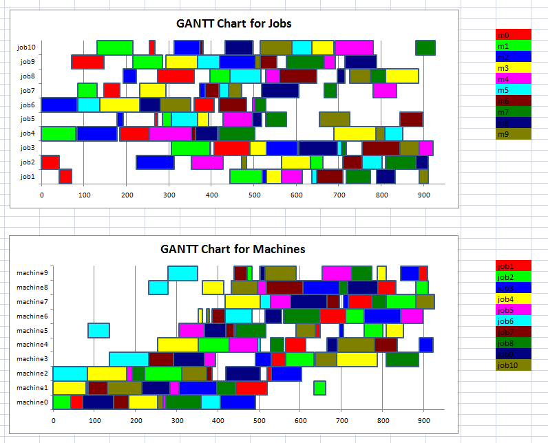
| MIP models to create time tables can be very difficult to solve. Here are some smaller instances. |